Laws tutorial

This tutorial provides simple examples on how to create learnable and non learnable laws into the iceflow model.

Let's say we have followed the classical workflow from ODINN, shown in the Forward simulation and Functional inversion tutorials. When we declare the Model type, we can specify the laws that we want to use in the iceflow model. Here we will briefly show how to do it. For more details you can check the Understanding the Law interface section.

using ODINN
using Plots
using Dates
using PlotlyJS

# Dummy parameters, only specifying the type of loss function to be used
params = Parameters(UDE = UDEparameters(empirical_loss_function = LossH()))

Sleipnir.Parameters{PhysicalParameters{Float64}, SimulationParameters{Int64, Float64, MeanDateVelocityMapping}, Hyperparameters{Float64, Int64}, SolverParameters{Float64, Int64}, UDEparameters{ContinuousAdjoint{Float64, Int64, DiscreteVJP{ADTypes.AutoMooncake{Nothing}}, EnzymeVJP}}, InversionParameters{Float64}}(PhysicalParameters{Float64}(900.0, 9.81, 1.0e-10, 1.0, 8.0e-17, 8.5e-20, 8.0e-17, 8.5e-20, 1.0, -25.0, 5.0e-18), SimulationParameters{Int64, Float64, MeanDateVelocityMapping}(true, true, true, true, 1.0, false, false, (2010.0, 2015.0), 0.08333333333333333, true, 4, "", false, Dict{String, String}(), "Farinotti19", MeanDateVelocityMapping(:nearest), 1), Hyperparameters{Float64, Int64}(1, 1, Float64[], Optim.BFGS{LineSearches.InitialStatic{Float64}, LineSearches.HagerZhang{Float64, Base.RefValue{Bool}}, Nothing, Float64, Optim.Flat}(LineSearches.InitialStatic{Float64}(1.0, false), LineSearches.HagerZhang{Float64, Base.RefValue{Bool}}(0.1, 0.9, Inf, 5.0, 1.0e-6, 0.66, 50, 0.1, 0, Base.RefValue{Bool}(false), nothing, false), nothing, 0.001, Optim.Flat()), 0.0, 50, 15), SolverParameters{Float64, Int64}(OrdinaryDiffEqLowStorageRK.RDPK3Sp35{typeof(OrdinaryDiffEqCore.trivial_limiter!), typeof(OrdinaryDiffEqCore.trivial_limiter!), Static.False}(OrdinaryDiffEqCore.trivial_limiter!, OrdinaryDiffEqCore.trivial_limiter!, static(false)), 1.0e-12, 0.08333333333333333, Float64[], false, true, 10, 100000), UDEparameters{ContinuousAdjoint{Float64, Int64, DiscreteVJP{ADTypes.AutoMooncake{Nothing}}, EnzymeVJP}}(SciMLSensitivity.GaussAdjoint{0, true, Val{:central}, SciMLSensitivity.EnzymeVJP}(SciMLSensitivity.EnzymeVJP(0), false), ADTypes.AutoEnzyme(), ContinuousAdjoint{Float64, Int64, DiscreteVJP{ADTypes.AutoMooncake{Nothing}}, EnzymeVJP}(DiscreteVJP{ADTypes.AutoMooncake{Nothing}}(ADTypes.AutoMooncake()), OrdinaryDiffEqLowStorageRK.RDPK3Sp35{typeof(OrdinaryDiffEqCore.trivial_limiter!), typeof(OrdinaryDiffEqCore.trivial_limiter!), Static.False}(OrdinaryDiffEqCore.trivial_limiter!, OrdinaryDiffEqCore.trivial_limiter!, static(false)), 1.0e-8, 1.0e-8, 0.08333333333333333, :Linear, 200, EnzymeVJP()), "AD+AD", LossH{L2Sum{Int64}}(L2Sum{Int64}(3)), :A, :identity), InversionParameters{Float64}([1.0], [0.0], [Inf], [1, 1], 0.001, 0.001, Optim.BFGS{LineSearches.InitialStatic{Float64}, LineSearches.HagerZhang{Float64, Base.RefValue{Bool}}, Nothing, Nothing, Optim.Flat}(LineSearches.InitialStatic{Float64}(1.0, false), LineSearches.HagerZhang{Float64, Base.RefValue{Bool}}(0.1, 0.9, Inf, 5.0, 1.0e-6, 0.66, 50, 0.1, 0, Base.RefValue{Bool}(false), nothing, false), nothing, nothing, Optim.Flat())))

Learnable laws

Learnable laws are laws that can be trained using a regressor (e.g., a linear regression function, a neural network, etc). They are used to map input variables to a target variable inside the iceflow model. In ODINN, we have implemented several learnable laws that can be used in the iceflow model.

nn_model = NeuralNetwork(params)

A_law = LawA(nn_model, params)

(:T,) -> Array{Float64, 0}   (↧@start  custom VJP  ✅ precomputed)

The output of the law definition above states that it maps the long term air temperature T to a float value which corresponds to the Glen coefficient A. It is defined as a neural network that takes as input T and returns A. The parameters θ of the neural network are learned during the inversion process, by minimizing the loss function given some target data (for this case the ice thickness).

As explained in the Sensitivity analysis section, ODINN computes vector-Jacobian products (VJPs) using AD in order to evaluate the gradient of the loss function. The part of the VJP concerning the law can be computed from different ways and it is possible to customize this, or use a default automatic differentiation backend. For this specific law, the VJPs are efficiently implemented and the user does not have to worry about this. The laws VJP customization tutorial provides a complete description of how this VJP computation can be customized.

The output above after A_law = LawA(nn_model, params) shows that the law is applied only once at the beginning of the simulation. Additionally, it inform us that custom VJPs used to compute the gradient are precomputed (that is, VJPs are computed before solving the adjoint iceflow PDE, refer to the laws VJP customization tutorial for more information).

It is then possible to visualize how the law integrates into the iceflow PDE:

model = Model(
    iceflow = SIA2Dmodel(params; A = A_law),
    mass_balance = TImodel1(params; DDF = 6.0 / 1000.0, acc_factor = 1.2 / 1000.0),
    regressors = (; A = nn_model)
)

**** Model ****

SIA2D iceflow equation  = ∇(D ∇S)  with D = U H̄
  and U = C (ρg)^(pq) H̄^(pq+1) ∇S^(p-1) + Γ H̄^(n+2) ∇S^(n-1)
      Γ = 2A (ρg)^n /(n+2)
      A: (:T,) -> Array{Float64, 0}   (↧@start  custom VJP  ✅ precomputed)
      C: ConstantLaw -> Array{Float64, 0}
      n: ConstantLaw -> Array{Float64, 0}
      p: ConstantLaw -> Array{Float64, 0}
      q: ConstantLaw -> Array{Float64, 0}
  where
      T => averaged_long_term_temperature

Temperature index mass balance model TImodel1
   DDF = 0.006
   acc_factor = 0.0012
Learnable components
  A: --- NeuralNetwork ---
    architecture:
      Chain(
          layer_1 = Dense(1 => 3, #101),                # 6 parameters
          layer_2 = Dense(3 => 10, #102),               # 40 parameters
          layer_3 = Dense(10 => 3, #103),               # 33 parameters
          layer_4 = Dense(3 => 1, σ),                   # 4 parameters
      )         # Total: 83 parameters,
                #        plus 0 states.
    θ: ComponentVector of length 83

***************

Non learnable laws

Non learnable laws are laws that are not trained using a regressor. They are used to map input variables to a target variable in the iceflow model, but they do not have any learnable parameters.

Example 1: Cuffey and Paterson (2010) 1-dimensional law

Here is a quick example also drawn from the functional inversion tutorial where a non learnable law has been used to generate the synthetic dataset.

A_law = CuffeyPaterson(scalar = true)

(:T,) -> Array{Float64, 0}   (↧@start  )

Note that this time since there is no learnable parameter, ODINN does not need to compute the VJPs.

model = Model(
    iceflow = SIA2Dmodel(params; A = A_law),
    mass_balance = TImodel1(params; DDF = 6.0 / 1000.0, acc_factor = 1.2 / 1000.0)
)

**** Model ****

SIA2D iceflow equation  = ∇(D ∇S)  with D = U H̄
  and U = C (ρg)^(pq) H̄^(pq+1) ∇S^(p-1) + Γ H̄^(n+2) ∇S^(n-1)
      Γ = 2A (ρg)^n /(n+2)
      A: (:T,) -> Array{Float64, 0}   (↧@start  )
      C: ConstantLaw -> Array{Float64, 0}
      n: ConstantLaw -> Array{Float64, 0}
      p: ConstantLaw -> Array{Float64, 0}
      q: ConstantLaw -> Array{Float64, 0}
  where
      T => averaged_long_term_temperature

Temperature index mass balance model TImodel1
   DDF = 0.006
   acc_factor = 0.0012
No learnable components
***************

In this ice flow model, the Glen coefficient A is defined by the CuffeyPaterson law, which is a non-learnable law that maps the long term air temperature T to A.

Example 2: Synthetic C (sliding) 2-dimensional law

In this example, we present a synthetic non-learnable law, that maps the basal sliding coefficient C to the surface topographical roughness and cumulative positive degree days (CPDDs).

rgi_paths = get_rgi_paths()

# Retrieving simulation data for the following glaciers
rgi_ids = ["RGI60-11.03638"]
δt = 1/12

0.08333333333333333

The key part here is the definition of the law inputs, which are the variables that will be used to compute the basal sliding coefficient C. In this case, we use the CPDD and the topographical roughness as inputs. As you can see, there are different options to customize the way the inputs are computed. For exampe, for the CPDD, we can specify a time window over which the CPDD is integrated. For the topographical roughness, we can specify a spatial window and the type of curvature to be used.

law_inputs = (; CPDD = iCPDD(window = Week(1)),
    topo_roughness = iTopoRough(window = 200.0, curvature_type = :variability))

(CPDD = CPDD: iCPDD{Dates.Week}(Dates.Week(1)), topo_roughness = topographic_roughness: iTopoRough{Float64}(200.0, :variability, :flow, :bed))

Then, we define the parameters as for any other simulation.

params = Parameters(
    simulation = SimulationParameters(
        use_MB = false,
        use_velocities = false,
        tspan = (2010.0, 2015.0),
        rgi_paths = rgi_paths,
        gridScalingFactor = 4 # We reduce the size of glacier for simulation
    ),
    solver = Huginn.SolverParameters(
        step = 1 / 12,
        progress = true
    )
)

Sleipnir.Parameters{PhysicalParameters{Float64}, SimulationParameters{Int64, Float64, MeanDateVelocityMapping}, Hyperparameters{Float64, Int64}, SolverParameters{Float64, Int64}, UDEparameters{ContinuousAdjoint{Float64, Int64, DiscreteVJP{ADTypes.AutoMooncake{Nothing}}, EnzymeVJP}}, InversionParameters{Float64}}(PhysicalParameters{Float64}(900.0, 9.81, 1.0e-10, 1.0, 8.0e-17, 8.5e-20, 8.0e-17, 8.5e-20, 1.0, -25.0, 5.0e-18), SimulationParameters{Int64, Float64, MeanDateVelocityMapping}(false, true, true, false, 1.0, false, false, (2010.0, 2015.0), 0.08333333333333333, true, 4, "", false, Dict("RGI60-11.00897" => "per_glacier/RGI60-11/RGI60-11.00/RGI60-11.00897", "RGI60-08.00213" => "per_glacier/RGI60-08/RGI60-08.00/RGI60-08.00213", "RGI60-08.00147" => "per_glacier/RGI60-08/RGI60-08.00/RGI60-08.00147", "RGI60-11.01270" => "per_glacier/RGI60-11/RGI60-11.01/RGI60-11.01270", "RGI60-11.03646" => "per_glacier/RGI60-11/RGI60-11.03/RGI60-11.03646", "RGI60-11.03232" => "per_glacier/RGI60-11/RGI60-11.03/RGI60-11.03232", "RGI60-01.22174" => "per_glacier/RGI60-01/RGI60-01.22/RGI60-01.22174", "RGI60-07.00274" => "per_glacier/RGI60-07/RGI60-07.00/RGI60-07.00274", "RGI60-03.04207" => "per_glacier/RGI60-03/RGI60-03.04/RGI60-03.04207", "RGI60-04.04351" => "per_glacier/RGI60-04/RGI60-04.04/RGI60-04.04351"…), "Farinotti19", MeanDateVelocityMapping(:nearest), 4), Hyperparameters{Float64, Int64}(1, 1, Float64[], Optim.BFGS{LineSearches.InitialStatic{Float64}, LineSearches.HagerZhang{Float64, Base.RefValue{Bool}}, Nothing, Float64, Optim.Flat}(LineSearches.InitialStatic{Float64}(1.0, false), LineSearches.HagerZhang{Float64, Base.RefValue{Bool}}(0.1, 0.9, Inf, 5.0, 1.0e-6, 0.66, 50, 0.1, 0, Base.RefValue{Bool}(false), nothing, false), nothing, 0.001, Optim.Flat()), 0.0, 50, 15), SolverParameters{Float64, Int64}(OrdinaryDiffEqLowStorageRK.RDPK3Sp35{typeof(OrdinaryDiffEqCore.trivial_limiter!), typeof(OrdinaryDiffEqCore.trivial_limiter!), Static.False}(OrdinaryDiffEqCore.trivial_limiter!, OrdinaryDiffEqCore.trivial_limiter!, static(false)), 1.0e-12, 0.08333333333333333, Float64[], false, true, 10, 100000), UDEparameters{ContinuousAdjoint{Float64, Int64, DiscreteVJP{ADTypes.AutoMooncake{Nothing}}, EnzymeVJP}}(SciMLSensitivity.GaussAdjoint{0, true, Val{:central}, SciMLSensitivity.EnzymeVJP}(SciMLSensitivity.EnzymeVJP(0), false), ADTypes.AutoEnzyme(), ContinuousAdjoint{Float64, Int64, DiscreteVJP{ADTypes.AutoMooncake{Nothing}}, EnzymeVJP}(DiscreteVJP{ADTypes.AutoMooncake{Nothing}}(ADTypes.AutoMooncake()), OrdinaryDiffEqLowStorageRK.RDPK3Sp35{typeof(OrdinaryDiffEqCore.trivial_limiter!), typeof(OrdinaryDiffEqCore.trivial_limiter!), Static.False}(OrdinaryDiffEqCore.trivial_limiter!, OrdinaryDiffEqCore.trivial_limiter!, static(false)), 1.0e-8, 1.0e-8, 0.08333333333333333, :Linear, 200, EnzymeVJP()), "AD+AD", MultiLoss{Tuple{LossH{L2Sum{Int64}}}, Vector{Float64}}((LossH{L2Sum{Int64}}(L2Sum{Int64}(3)),), [1.0]), :A, :identity), InversionParameters{Float64}([1.0], [0.0], [Inf], [1, 1], 0.001, 0.001, Optim.BFGS{LineSearches.InitialStatic{Float64}, LineSearches.HagerZhang{Float64, Base.RefValue{Bool}}, Nothing, Nothing, Optim.Flat}(LineSearches.InitialStatic{Float64}(1.0, false), LineSearches.HagerZhang{Float64, Base.RefValue{Bool}}(0.1, 0.9, Inf, 5.0, 1.0e-6, 0.66, 50, 0.1, 0, Base.RefValue{Bool}(false), nothing, false), nothing, nothing, Optim.Flat())))

When declaring the model, we will indicate that the basal sliding coefficient C will be simulated by the SyntheticC law, which takes as input the parameters and the law inputs we defined before.

model = Huginn.Model(
    iceflow = SIA2Dmodel(params; C = SyntheticC(params; inputs = law_inputs)),
    mass_balance = nothing
)

**** Model ****

SIA2D iceflow equation  = ∇(D ∇S)  with D = U H̄
  and U = C (ρg)^(pq) H̄^(pq+1) ∇S^(p-1) + Γ H̄^(n+2) ∇S^(n-1)
      Γ = 2A (ρg)^n /(n+2)
      A: ConstantLaw -> Array{Float64, 0}
      C: (:CPDD, :topo_roughness) -> Matrix{Float64}   (↧0.019  )
      n: ConstantLaw -> Array{Float64, 0}
      p: ConstantLaw -> Array{Float64, 0}
      q: ConstantLaw -> Array{Float64, 0}
  where
      CPDD => CPDD
      topo_roughness => topographic_roughness

nothing
No learnable components
***************

We retrieve some glaciers for the simulation

glaciers = initialize_glaciers(rgi_ids, params)

1-element Vector{Glacier2D} distributed over regions 11 (x1)
RGI60-11.03638

Time snapshots for transient inversion

tstops = collect(2010:δt:2015)

61-element Vector{Float64}:
 2010.0
 2010.0833333333333
 2010.1666666666667
 2010.25
 2010.3333333333333
 2010.4166666666667
 2010.5
 2010.5833333333333
 2010.6666666666667
 2010.75
    ⋮
 2014.3333333333333
 2014.4166666666667
 2014.5
 2014.5833333333333
 2014.6666666666667
 2014.75
 2014.8333333333333
 2014.9166666666667
 2015.0

Then, we can run the generate_ground_truth_prediction function to simulate the glacier evolution using the defined law.

prediction = generate_ground_truth_prediction(glaciers, params, model, tstops)

Prediction{Sleipnir.ModelCache{SIA2DCache{Float64, Int64, ScalarCacheNoVJP, MatrixCacheNoVJP, ScalarCacheNoVJP, ScalarCacheNoVJP, ScalarCacheNoVJP, Array{Float64, 0}, Array{Float64, 0}, ScalarCacheNoVJP, ScalarCacheNoVJP}, Nothing}}(Sleipnir.Model{SIA2Dmodel{Float64, ConstantLaw{ScalarCacheNoVJP, Huginn.var"#7#8"}, Law{MatrixCacheNoVJP, Sleipnir.GenInputsAndApply{@NamedTuple{CPDD::iCPDD{Dates.Week}, topo_roughness::iTopoRough{Float64}}, Huginn.var"#41#44"{Sleipnir.Parameters{PhysicalParameters{Float64}, SimulationParameters{Int64, Float64, MeanDateVelocityMapping}, Hyperparameters{Float64, Int64}, SolverParameters{Float64, Int64}, UDEparameters{ContinuousAdjoint{Float64, Int64, DiscreteVJP{ADTypes.AutoMooncake{Nothing}}, EnzymeVJP}}, InversionParameters{Float64}}}}, Sleipnir.GenInputsAndApply{@NamedTuple{CPDD::iCPDD{Dates.Week}, topo_roughness::iTopoRough{Float64}}, typeof(Sleipnir.emptyVJPWithInputs)}, Sleipnir.GenInputsAndApply{@NamedTuple{CPDD::iCPDD{Dates.Week}, topo_roughness::iTopoRough{Float64}}, typeof(Sleipnir.emptyVJPWithInputs)}, Huginn.var"#43#46", Float64, Sleipnir.GenInputsAndApply{@NamedTuple{CPDD::iCPDD{Dates.Week}, topo_roughness::iTopoRough{Float64}}, typeof(Sleipnir.emptyPrepVJPWithInputs)}, DIVJP}, ConstantLaw{ScalarCacheNoVJP, Huginn.var"#11#12"}, ConstantLaw{ScalarCacheNoVJP, Huginn.var"#13#14"}, ConstantLaw{ScalarCacheNoVJP, Huginn.var"#15#16"}, NullLaw, NullLaw}, Nothing, Nothing}(SIA2D iceflow equation  = ∇(D ∇S)  with D = U H̄
  and U = C (ρg)^(pq) H̄^(pq+1) ∇S^(p-1) + Γ H̄^(n+2) ∇S^(n-1)
      Γ = 2A (ρg)^n /(n+2)
      A: ConstantLaw -> Array{Float64, 0}
      C: (:CPDD, :topo_roughness) -> Matrix{Float64}   (↧0.019  )
      n: ConstantLaw -> Array{Float64, 0}
      p: ConstantLaw -> Array{Float64, 0}
      q: ConstantLaw -> Array{Float64, 0}
  where
      CPDD => CPDD
      topo_roughness => topographic_roughness
, nothing, nothing), nothing, 1-element Vector{AbstractGlacier} distributed over regions 11 (x1)
RGI60-11.03638
, Sleipnir.Parameters{PhysicalParameters{Float64}, SimulationParameters{Int64, Float64, MeanDateVelocityMapping}, Hyperparameters{Float64, Int64}, SolverParameters{Float64, Int64}, UDEparameters{ContinuousAdjoint{Float64, Int64, DiscreteVJP{ADTypes.AutoMooncake{Nothing}}, EnzymeVJP}}, InversionParameters{Float64}}(PhysicalParameters{Float64}(900.0, 9.81, 1.0e-10, 1.0, 8.0e-17, 8.5e-20, 8.0e-17, 8.5e-20, 1.0, -25.0, 5.0e-18), SimulationParameters{Int64, Float64, MeanDateVelocityMapping}(false, true, true, false, 1.0, false, false, (2010.0, 2015.0), 0.08333333333333333, true, 4, "", false, Dict("RGI60-11.00897" => "per_glacier/RGI60-11/RGI60-11.00/RGI60-11.00897", "RGI60-08.00213" => "per_glacier/RGI60-08/RGI60-08.00/RGI60-08.00213", "RGI60-08.00147" => "per_glacier/RGI60-08/RGI60-08.00/RGI60-08.00147", "RGI60-11.01270" => "per_glacier/RGI60-11/RGI60-11.01/RGI60-11.01270", "RGI60-11.03646" => "per_glacier/RGI60-11/RGI60-11.03/RGI60-11.03646", "RGI60-11.03232" => "per_glacier/RGI60-11/RGI60-11.03/RGI60-11.03232", "RGI60-01.22174" => "per_glacier/RGI60-01/RGI60-01.22/RGI60-01.22174", "RGI60-07.00274" => "per_glacier/RGI60-07/RGI60-07.00/RGI60-07.00274", "RGI60-03.04207" => "per_glacier/RGI60-03/RGI60-03.04/RGI60-03.04207", "RGI60-04.04351" => "per_glacier/RGI60-04/RGI60-04.04/RGI60-04.04351"…), "Farinotti19", MeanDateVelocityMapping(:nearest), 4), Hyperparameters{Float64, Int64}(1, 1, Float64[], Optim.BFGS{LineSearches.InitialStatic{Float64}, LineSearches.HagerZhang{Float64, Base.RefValue{Bool}}, Nothing, Float64, Optim.Flat}(LineSearches.InitialStatic{Float64}(1.0, false), LineSearches.HagerZhang{Float64, Base.RefValue{Bool}}(0.1, 0.9, Inf, 5.0, 1.0e-6, 0.66, 50, 0.1, 0, Base.RefValue{Bool}(false), nothing, false), nothing, 0.001, Optim.Flat()), 0.0, 50, 15), SolverParameters{Float64, Int64}(OrdinaryDiffEqLowStorageRK.RDPK3Sp35{typeof(OrdinaryDiffEqCore.trivial_limiter!), typeof(OrdinaryDiffEqCore.trivial_limiter!), Static.False}(OrdinaryDiffEqCore.trivial_limiter!, OrdinaryDiffEqCore.trivial_limiter!, static(false)), 1.0e-12, 0.08333333333333333, Float64[], false, true, 10, 100000), UDEparameters{ContinuousAdjoint{Float64, Int64, DiscreteVJP{ADTypes.AutoMooncake{Nothing}}, EnzymeVJP}}(SciMLSensitivity.GaussAdjoint{0, true, Val{:central}, SciMLSensitivity.EnzymeVJP}(SciMLSensitivity.EnzymeVJP(0), false), ADTypes.AutoEnzyme(), ContinuousAdjoint{Float64, Int64, DiscreteVJP{ADTypes.AutoMooncake{Nothing}}, EnzymeVJP}(DiscreteVJP{ADTypes.AutoMooncake{Nothing}}(ADTypes.AutoMooncake()), OrdinaryDiffEqLowStorageRK.RDPK3Sp35{typeof(OrdinaryDiffEqCore.trivial_limiter!), typeof(OrdinaryDiffEqCore.trivial_limiter!), Static.False}(OrdinaryDiffEqCore.trivial_limiter!, OrdinaryDiffEqCore.trivial_limiter!, static(false)), 1.0e-8, 1.0e-8, 0.08333333333333333, :Linear, 200, EnzymeVJP()), "AD+AD", MultiLoss{Tuple{LossH{L2Sum{Int64}}}, Vector{Float64}}((LossH{L2Sum{Int64}}(L2Sum{Int64}(3)),), [1.0]), :A, :identity), InversionParameters{Float64}([1.0], [0.0], [Inf], [1, 1], 0.001, 0.001, Optim.BFGS{LineSearches.InitialStatic{Float64}, LineSearches.HagerZhang{Float64, Base.RefValue{Bool}}, Nothing, Nothing, Optim.Flat}(LineSearches.InitialStatic{Float64}(1.0, false), LineSearches.HagerZhang{Float64, Base.RefValue{Bool}}(0.1, 0.9, Inf, 5.0, 1.0e-6, 0.66, 50, 0.1, 0, Base.RefValue{Bool}(false), nothing, false), nothing, nothing, Optim.Flat()))), Sleipnir.Results[])

Importantly, we provide the plot_law function to visualize 2-dimensional laws in 3D. This is especially useful when exploring the behaviour of laws with respect to different proxies, and to better understand learnable laws and their drivers.

fig = plot_law(prediction.model.iceflow.C, prediction, law_inputs, nothing);

Since we are in the documentation it is not possible to have an interactive plot but if you reproduce this example locally, you can run the line above without ";" and you can skip the lines hereafter. This will open an interactive window with a 3D plot that you can rotate.

folder = "laws_plots"
mkpath(folder)
filepath = joinpath(folder, "3d_plot.png")
PlotlyJS.savefig(fig, filepath);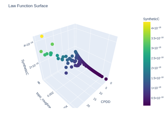

This page was generated using Literate.jl.